Prepare the datasets
movies = as.data.frame(ggplot2movies::movies)
head(movies, 3)| title | year | length | budget | rating | votes | r1 | r2 | r3 | r4 | ⋯ | r9 | r10 | mpaa | Action | Animation | Comedy | Drama | Documentary | Romance | Short | |
|---|---|---|---|---|---|---|---|---|---|---|---|---|---|---|---|---|---|---|---|---|---|
| <chr> | <int> | <int> | <int> | <dbl> | <int> | <dbl> | <dbl> | <dbl> | <dbl> | ⋯ | <dbl> | <dbl> | <chr> | <int> | <int> | <int> | <int> | <int> | <int> | <int> | |
| 1 | $ | 1971 | 121 | NA | 6.4 | 348 | 4.5 | 4.5 | 4.5 | 4.5 | ⋯ | 4.5 | 4.5 | 0 | 0 | 1 | 1 | 0 | 0 | 0 | |
| 2 | $1000 a Touchdown | 1939 | 71 | NA | 6.0 | 20 | 0.0 | 14.5 | 4.5 | 24.5 | ⋯ | 4.5 | 14.5 | 0 | 0 | 1 | 0 | 0 | 0 | 0 | |
| 3 | $21 a Day Once a Month | 1941 | 7 | NA | 8.2 | 5 | 0.0 | 0.0 | 0.0 | 0.0 | ⋯ | 24.5 | 24.5 | 0 | 1 | 0 | 0 | 0 | 0 | 1 |
genres = colnames(movies)[18:24]
genres- ‘Action’
- ‘Animation’
- ‘Comedy’
- ‘Drama’
- ‘Documentary’
- ‘Romance’
- ‘Short’
Convert the genre indicator columns to use boolean values:
| 1 | 2 | 3 | |
|---|---|---|---|
| Action | FALSE | FALSE | FALSE |
| Animation | FALSE | FALSE | TRUE |
| Comedy | TRUE | TRUE | FALSE |
| Drama | TRUE | FALSE | FALSE |
| Documentary | FALSE | FALSE | FALSE |
| Romance | FALSE | FALSE | FALSE |
| Short | FALSE | FALSE | TRUE |
To keep the examples fast to compile we will operate on a subset of the movies with complete data:
movies[movies$mpaa == '', 'mpaa'] = NA
movies = na.omit(movies)
Utility for changing output parameters in Jupyter notebooks (IRKernel kernel), not relevant if using RStudio or scripting R from terminal:
set_size = function(w, h, factor=1.5) {
    s = 1 * factor
    options(
        repr.plot.width=w * s,
        repr.plot.height=h * s,
        repr.plot.res=100 / factor,
        jupyter.plot_mimetypes='image/png',
        jupyter.plot_scale=1
    )
}
0. Basic usage
There are two required arguments:
- the first argument is expected to be a dataframe with both group indicator variables and covariates,
- the second argument specifies a list with names of column which indicate the group membership.
Additional arguments can be provided, such as name
(specifies xlab() for intersection matrix) or
width_ratio (specifies how much space should be occupied by
the set size panel). Other such arguments are discussed at length later
in this document.
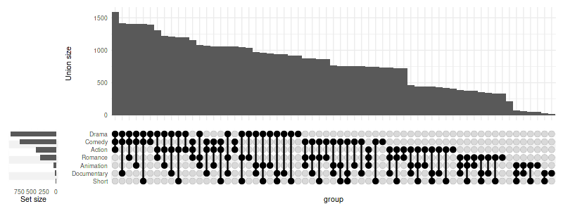
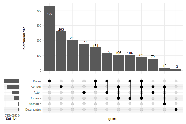
set_size(8, 3)
upset(movies, genres, name='genre', width_ratio=0.1)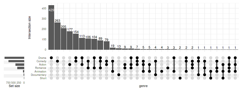
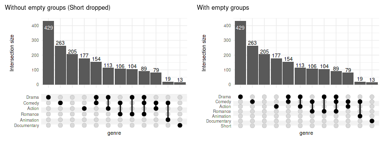
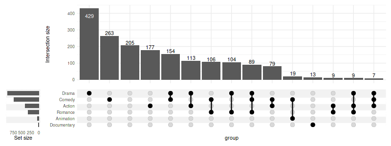
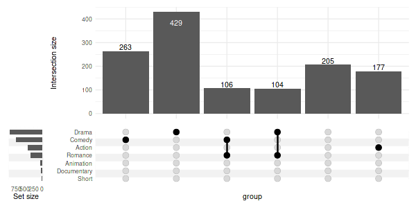
0.1 Selecting intersections
We will focus on the intersections with at least ten members
(min_size=10) and on a few variables which are
significantly different between the intersections (see 2. Running
statistical tests).
When using min_size, the empty groups will be skipped by
default (e.g. Short movies would have no overlap with size of
10). To keep all groups pass keep_empty_groups=TRUE:
set_size(8, 3)
(
    upset(movies, genres, name='genre', width_ratio=0.1, min_size=10, wrap=TRUE, set_sizes=FALSE)
    + ggtitle('Without empty groups (Short dropped)')
    +    # adding plots is possible thanks to patchwork
    upset(movies, genres, name='genre', width_ratio=0.1, min_size=10, keep_empty_groups=TRUE, wrap=TRUE, set_sizes=FALSE)
    + ggtitle('With empty groups')
)
When empty columns are detected a warning will be issued. The silence
it, pass warn_when_dropping_groups=FALSE. Complimentary
max_size can be used in tandem.
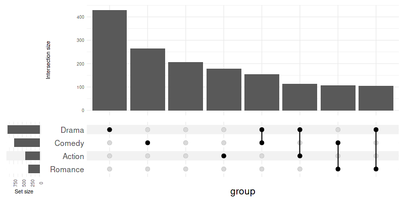
You can also select intersections by degree (min_degree
and max_degree):
set_size(8, 3)
upset(
    movies, genres, width_ratio=0.1,
    min_degree=3,
)
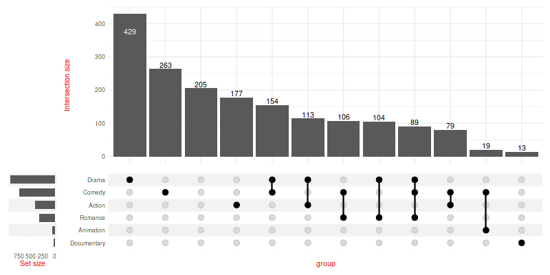
Or request a constant number of intersections with
n_intersections:
set_size(8, 3)
upset(
    movies, genres, width_ratio=0.1,
    n_intersections=15
)
0.2 Region selection modes
There are four modes defining the regions of interest on corresponding Venn diagram:
-
exclusive_intersectionregion: intersection elements that belong to the sets defining the intersection but not to any other set (alias: distinct), default -
inclusive_intersectionregion: intersection elements that belong to the sets defining the intersection including overlaps with other sets (alias: intersect) -
exclusive_unionregion: union elements that belong to the sets defining the union, excluding those overlapping with any other set -
inclusive_unionregion: union elements that belong to the sets defining the union, including those overlapping with any other set (alias: union)
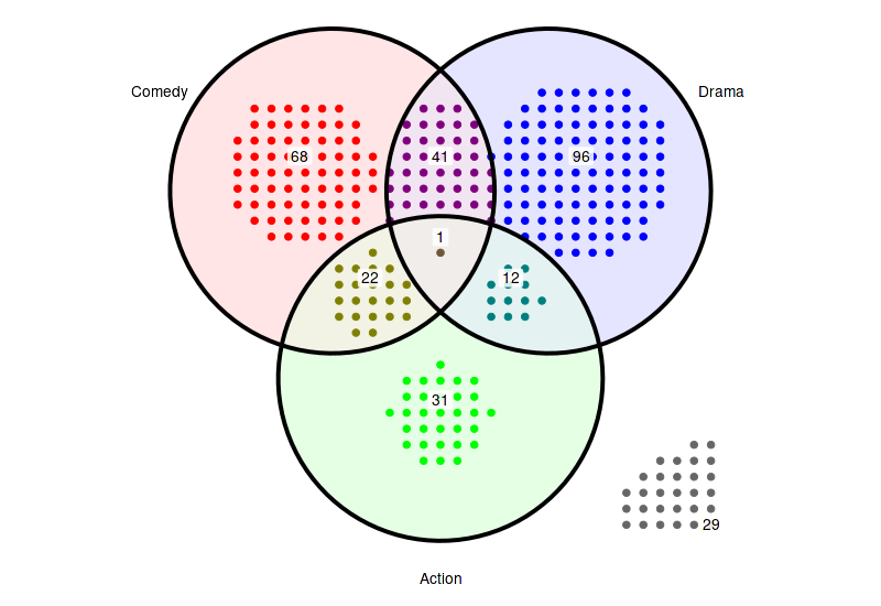
Example: given three sets \(A\), \(B\) and \(C\) with number of elements defined by the Venn diagram below
abc_data = create_upset_abc_example()

abc_venn = (
    ggplot(arrange_venn(abc_data))
    + coord_fixed()
    + theme_void()
    + scale_color_venn_mix(abc_data)
)

(
    abc_venn
    + geom_venn_region(data=abc_data, alpha=0.05)
    + geom_point(aes(x=x, y=y, color=region), size=1)
    + geom_venn_circle(abc_data)
    + geom_venn_label_set(abc_data, aes(label=region))
    + geom_venn_label_region(
        abc_data, aes(label=size),
        outwards_adjust=1.75,
        position=position_nudge(y=0.2)
    )
    + scale_fill_venn_mix(abc_data, guide='none')
)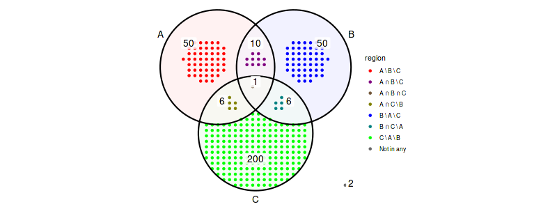
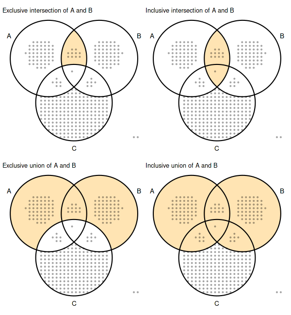
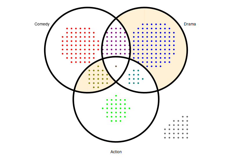
For the above sets \(A\) and \(B\) the region selection modes correspond to region of Venn diagram defined as follows:
- exclusive intersection: \((A \cap B) \setminus C\)
- inclusive intersection: \(A \cap B\)
- exclusive union: \((A \cup B) \setminus C\)
- inclusive union: \(A \cup B\)
and have the total number of elements as in the table below:
| members mode | exclusive int. | inclusive int. | exclusive union | inclusive union |
|---|---|---|---|---|
| (A, B) | 10 | 11 | 110 | 123 |
| (A, C) == (B, C) | 6 | 7 | 256 | 273 |
| (A) == (B) | 50 | 67 | 50 | 67 |
| (C) | 200 | 213 | 200 | 213 |
| (A, B, C) | 1 | 1 | 323 | 323 |
| () | 2 | 2 | 2 | 2 |
set_size(6, 6.5)
simple_venn = (
    abc_venn
    + geom_venn_region(data=abc_data, alpha=0.3)
    + geom_point(aes(x=x, y=y), size=0.75, alpha=0.3)
    + geom_venn_circle(abc_data)
    + geom_venn_label_set(abc_data, aes(label=region), outwards_adjust=2.55)
)
highlight = function(regions) scale_fill_venn_mix(
    abc_data, guide='none', highlight=regions, inactive_color='NA'
)

(
    (
        simple_venn + highlight(c('A-B')) + labs(title='Exclusive intersection of A and B')
        | simple_venn + highlight(c('A-B', 'A-B-C')) + labs(title='Inclusive intersection of A and B')
    ) /
    (
        simple_venn + highlight(c('A-B', 'A', 'B')) + labs(title='Exclusive union of A and B')
        | simple_venn + highlight(c('A-B', 'A-B-C', 'A', 'B', 'A-C', 'B-C')) + labs(title='Inclusive union of A and B')
    )
)
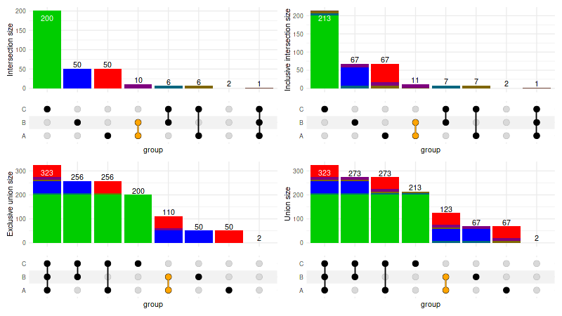
When customizing the intersection_size() it is important
to adjust the mode accordingly, as it defaults to
exclusive_intersection and cannot be automatically deduced
when user customizations are being applied:
set_size(8, 4.5)
abc_upset = function(mode) upset(
    abc_data, c('A', 'B', 'C'), mode=mode, set_sizes=FALSE,
    encode_sets=FALSE,
    queries=list(upset_query(intersect=c('A', 'B'), color='orange')),
    base_annotations=list(
        'Size'=(
            intersection_size(
                mode=mode,
                mapping=aes(fill=exclusive_intersection),
                size=0,
                text=list(check_overlap=TRUE)
            ) + scale_fill_venn_mix(
                data=abc_data,
                guide='none',
                colors=c('A'='red', 'B'='blue', 'C'='green3')
            )
        )
    )
)

(
    (abc_upset('exclusive_intersection') | abc_upset('inclusive_intersection'))
    /
    (abc_upset('exclusive_union') | abc_upset('inclusive_union'))
)
0.3 Displaying all intersections
To display all possible intersections (rather than only the observed
ones) use intersections='all'.
Note 1: it is usually desired to filter all the
possible intersections down with max_degree and/or
min_degree to avoid generating all combinations as those
can easily use up all available RAM memory when dealing with multiple
sets (e.g. all human genes) due to sheer number of possible
combinations
Note 2: using intersections='all' is
only reasonable for mode different from the default exclusive
intersection.
set_size(8, 3)
upset(
    movies, genres,
    width_ratio=0.1,
    min_size=10,
    mode='inclusive_union',
    base_annotations=list('Size'=(intersection_size(counts=FALSE, mode='inclusive_union'))),
    intersections='all',
    max_degree=3
)
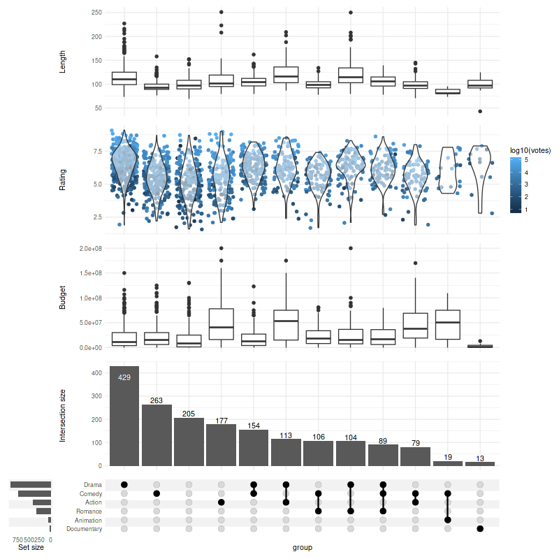
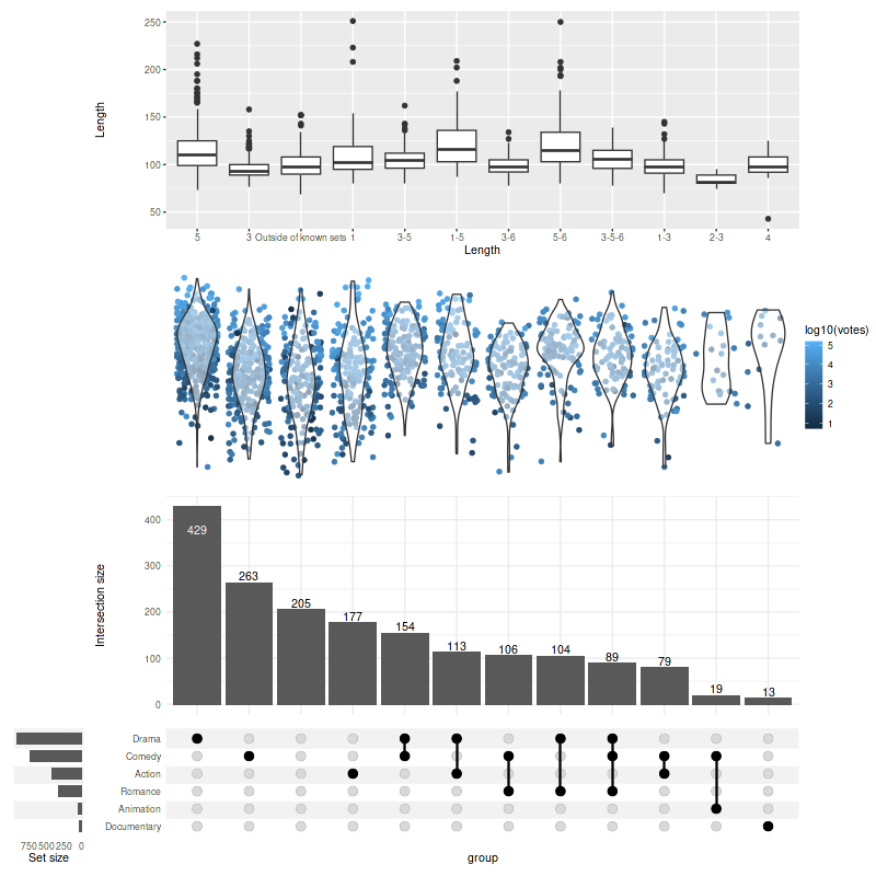
1. Adding components
We can add multiple annotation components (also called panels) using one of the three methods demonstrated below:
set_size(8, 8)

set.seed(0)   # keep the same jitter for identical plots

upset(
    movies,
    genres,
    annotations = list(
        # 1st method - passing list:
        'Length'=list(
            aes=aes(x=intersection, y=length),
            # provide a list if you wish to add several geoms
            geom=geom_boxplot(na.rm=TRUE)
        ),
        # 2nd method - using ggplot
        'Rating'=(
            # note that aes(x=intersection) is supplied by default and can be skipped
            ggplot(mapping=aes(y=rating))
            # checkout ggbeeswarm::geom_quasirandom for better results!
            + geom_jitter(aes(color=log10(votes)), na.rm=TRUE)
            + geom_violin(alpha=0.5, na.rm=TRUE)
        ),
        # 3rd method - using `upset_annotate` shorthand
        'Budget'=upset_annotate('budget', geom_boxplot(na.rm=TRUE))
    ),
    min_size=10,
    width_ratio=0.1
)
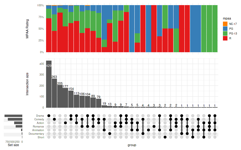
You can also use barplots to demonstrate differences in proportions of categorical variables:
set_size(8, 5)

upset(
    movies,
    genres,
    annotations = list(
        'MPAA Rating'=(
            ggplot(mapping=aes(fill=mpaa))
            + geom_bar(stat='count', position='fill')
            + scale_y_continuous(labels=scales::percent_format())
            + scale_fill_manual(values=c(
                'R'='#E41A1C', 'PG'='#377EB8',
                'PG-13'='#4DAF4A', 'NC-17'='#FF7F00'
            ))
            + ylab('MPAA Rating')
        )
    ),
    width_ratio=0.1
)
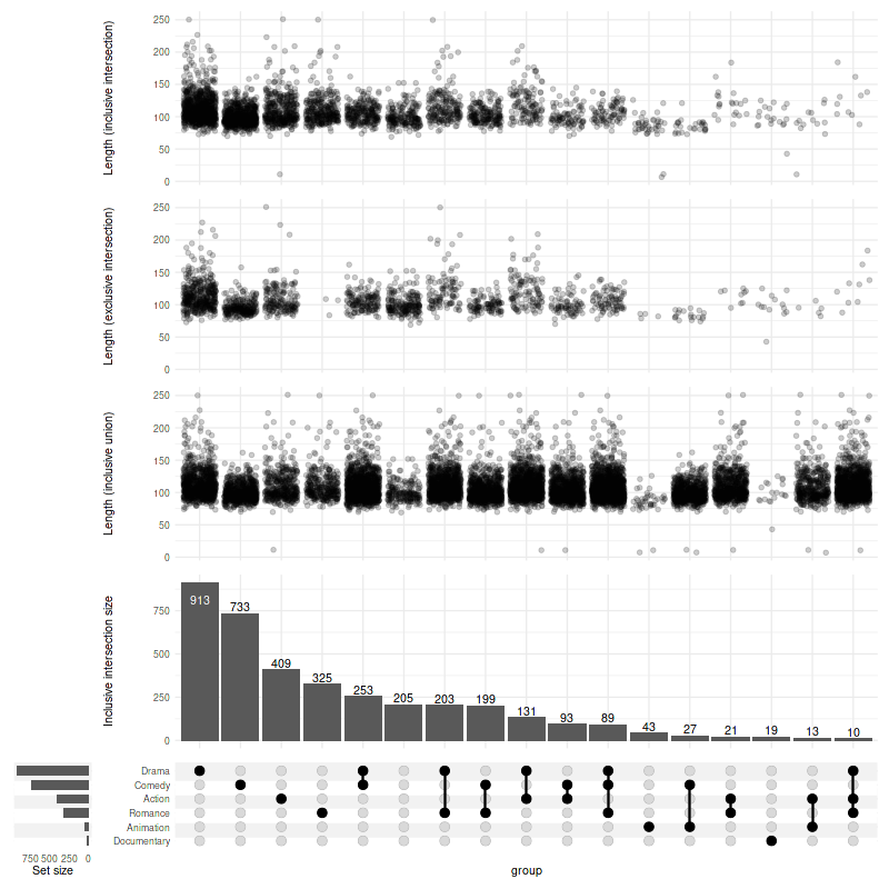
1.1. Changing modes in annotations
Use upset_mode to change the mode of the annotation:
set_size(8, 8)
set.seed(0)
upset(
    movies,
    genres,
    mode='inclusive_intersection',
    annotations = list(
        # if not specified, the mode will follow the mode set in `upset()` call (here: `inclusive_intersection`)
        'Length (inclusive intersection)'=(
            ggplot(mapping=aes(y=length))
            + geom_jitter(alpha=0.2, na.rm=TRUE)
        ),
        'Length (exclusive intersection)'=(
            ggplot(mapping=aes(y=length))
            + geom_jitter(alpha=0.2, na.rm=TRUE)
            + upset_mode('exclusive_intersection')
        ),
        'Length (inclusive union)'=(
            ggplot(mapping=aes(y=length))
            + geom_jitter(alpha=0.2, na.rm=TRUE)
            + upset_mode('inclusive_union')
        )
    ),
    min_size=10,
    width_ratio=0.1
)
2. Running statistical tests
upset_test(movies, genres)[1] "year, length, budget, rating, votes, r1, r2, r3, r4, r5, r6, r7, r8, r9, r10, mpaa differ significantly between intersections"| variable | p.value | statistic | test | fdr | |
|---|---|---|---|---|---|
| <chr> | <dbl> | <dbl> | <chr> | <dbl> | |
| length | length | 6.511525e-71 | 422.88444 | Kruskal-Wallis rank sum test | 1.106959e-69 |
| rating | rating | 1.209027e-46 | 301.72764 | Kruskal-Wallis rank sum test | 1.027673e-45 |
| budget | budget | 3.899860e-44 | 288.97476 | Kruskal-Wallis rank sum test | 2.209921e-43 |
| r8 | r8 | 9.900004e-39 | 261.28815 | Kruskal-Wallis rank sum test | 4.207502e-38 |
| mpaa | mpaa | 3.732200e-35 | 242.77939 | Kruskal-Wallis rank sum test | 1.268948e-34 |
| r9 | r9 | 1.433256e-30 | 218.78160 | Kruskal-Wallis rank sum test | 4.060891e-30 |
| r1 | r1 | 2.211600e-23 | 180.32740 | Kruskal-Wallis rank sum test | 5.371029e-23 |
| r4 | r4 | 1.008119e-18 | 154.62772 | Kruskal-Wallis rank sum test | 2.142254e-18 |
| r3 | r3 | 2.568227e-17 | 146.70217 | Kruskal-Wallis rank sum test | 4.851095e-17 |
| r5 | r5 | 9.823827e-16 | 137.66310 | Kruskal-Wallis rank sum test | 1.670051e-15 |
| r7 | r7 | 9.201549e-14 | 126.19243 | Kruskal-Wallis rank sum test | 1.422058e-13 |
| r2 | r2 | 2.159955e-13 | 124.00604 | Kruskal-Wallis rank sum test | 3.059936e-13 |
| r10 | r10 | 1.283470e-11 | 113.38113 | Kruskal-Wallis rank sum test | 1.678384e-11 |
| votes | votes | 2.209085e-10 | 105.79588 | Kruskal-Wallis rank sum test | 2.682460e-10 |
| r6 | r6 | 3.779129e-05 | 70.80971 | Kruskal-Wallis rank sum test | 4.283013e-05 |
| year | year | 2.745818e-02 | 46.55972 | Kruskal-Wallis rank sum test | 2.917431e-02 |
| title | title | 2.600003e-01 | 34.53375 | Kruskal-Wallis rank sum test | 2.600003e-01 |
Kruskal-Wallis rank sum test is not always the best
choice.
You can either change the test for:
- all the variables (
test=your.test), or - specific variables (using
tests=list(variable=some.test)argument)
The tests are called with
(formula=variable ~ intersection, data) signature, such as
accepted by kruskal.test. The result is expected to be a
list with following members:
p.valuestatisticmethod
It is easy to adapt tests which do not obey this signature/output convention; for example the Chi-squared test and anova can be wrapped with two-line functions as follows:
chisq_from_formula = function(formula, data) {
    chisq.test(
        ftable(formula, data)
    )
}

anova_single = function(formula, data) {
    result = summary(aov(formula, data))
    list(
        p.value=result[[1]][['Pr(>F)']][[1]],
        method='Analysis of variance Pr(>F)',
        statistic=result[[1]][['F value']][[1]]
    )
}

custom_tests = list(
    mpaa=chisq_from_formula,
    budget=anova_single
)
head(upset_test(movies, genres, tests=custom_tests))Warning message in chisq.test(ftable(formula, data)):
“Chi-squared approximation may be incorrect”
[1] "year, length, budget, rating, votes, r1, r2, r3, r4, r5, r6, r7, r8, r9, r10, mpaa differ significantly between intersections"| variable | p.value | statistic | test | fdr | |
|---|---|---|---|---|---|
| <chr> | <dbl> | <dbl> | <chr> | <dbl> | |
| length | length | 6.511525e-71 | 422.88444 | Kruskal-Wallis rank sum test | 1.106959e-69 |
| budget | budget | 1.348209e-60 | 13.66395 | Analysis of variance Pr(>F) | 1.145977e-59 |
| rating | rating | 1.209027e-46 | 301.72764 | Kruskal-Wallis rank sum test | 6.851151e-46 |
| mpaa | mpaa | 9.799097e-42 | 406.33814 | Pearson’s Chi-squared test | 4.164616e-41 |
| r8 | r8 | 9.900004e-39 | 261.28815 | Kruskal-Wallis rank sum test | 3.366002e-38 |
| r9 | r9 | 1.433256e-30 | 218.78160 | Kruskal-Wallis rank sum test | 4.060891e-30 |
Many tests will require at least two observations in each group. You
can skip intersections with less than two members with
min_size=2.
bartlett_results = suppressWarnings(upset_test(movies, genres, test=bartlett.test, min_size=2))
tail(bartlett_results)
[1] "NA, year, length, budget, rating, votes, r1, r2, r3, r4, r5, r6, r7, r8, r9, r10, NA differ significantly between intersections"| variable | p.value | statistic | test | fdr | |
|---|---|---|---|---|---|
| <chr> | <dbl> | <dbl> | <chr> | <dbl> | |
| year | year | 1.041955e-67 | 386.53699 | Bartlett test of homogeneity of variances | 1.302444e-67 |
| length | length | 3.982729e-67 | 383.70148 | Bartlett test of homogeneity of variances | 4.595457e-67 |
| budget | budget | 7.637563e-50 | 298.89911 | Bartlett test of homogeneity of variances | 8.183103e-50 |
| rating | rating | 3.980194e-06 | 66.63277 | Bartlett test of homogeneity of variances | 3.980194e-06 |
| title | title | NA | NA | Bartlett test of homogeneity of variances | NA |
| mpaa | mpaa | NA | NA | Bartlett test of homogeneity of variances | NA |
2.1 Ignore specific variables
You may want to exclude variables which are:
- highly correlated and therefore interfering with the FDR calculation, or
- simply irrelevant
In the movies example, the title variable is not a reasonable thing to compare. We can ignore it using:
# note: title no longer present
rownames(upset_test(movies, genres, ignore=c('title')))
[1] "year, length, budget, rating, votes, r1, r2, r3, r4, r5, r6, r7, r8, r9, r10, mpaa differ significantly between intersections"- ‘length’
- ‘rating’
- ‘budget’
- ‘r8’
- ‘mpaa’
- ‘r9’
- ‘r1’
- ‘r4’
- ‘r3’
- ‘r5’
- ‘r7’
- ‘r2’
- ‘r10’
- ‘votes’
- ‘r6’
- ‘year’
3. Adjusting “Intersection size”
3.1 Counts
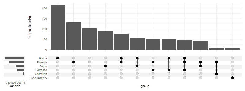
The counts over the bars can be disabled:
set_size(8, 3)

upset(
    movies,
    genres,
    base_annotations=list(
        'Intersection size'=intersection_size(counts=FALSE)
    ),
    min_size=10,
    width_ratio=0.1
)
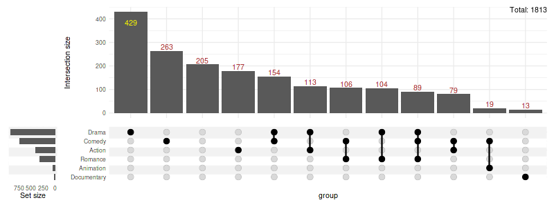
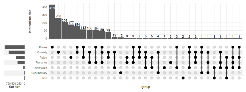
The colors can be changed, and additional annotations added:
set_size(8, 3)

upset(
    movies,
    genres,
    base_annotations=list(
        'Intersection size'=intersection_size(
            text_colors=c(
                on_background='brown', on_bar='yellow'
            )
        )
        + annotate(
            geom='text', x=Inf, y=Inf,
            label=paste('Total:', nrow(movies)),
            vjust=1, hjust=1
        )
        + ylab('Intersection size')
    ),
    min_size=10,
    width_ratio=0.1
)
Any parameter supported by geom_text can be passed in
text list:
set_size(8, 3)

upset(
    movies,
    genres,
    base_annotations=list(
        'Intersection size'=intersection_size(
            text=list(
                vjust=-0.1,
                hjust=-0.1,
                angle=45
            )
        )
    ),
    min_size=10,
    width_ratio=0.1
)
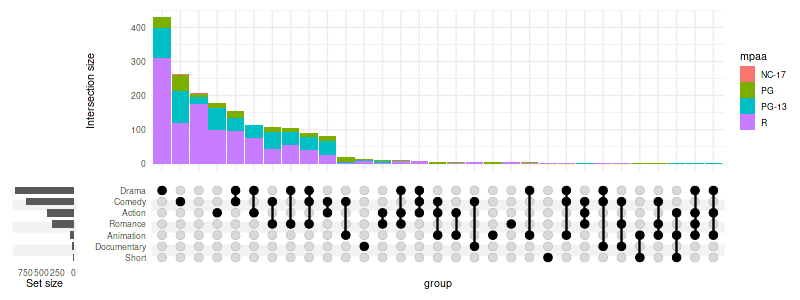
3.2 Fill the bars
set_size(8, 3)

upset(
    movies,
    genres,
    base_annotations=list(
        'Intersection size'=intersection_size(
            counts=FALSE,
            mapping=aes(fill=mpaa)
        )
    ),
    width_ratio=0.1
)
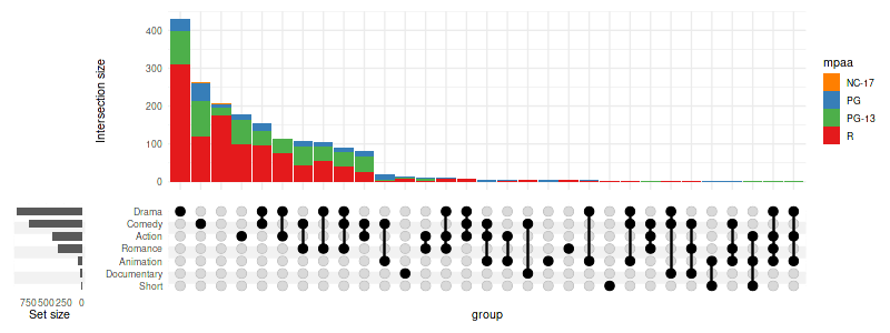
set_size(8, 3)
upset(
    movies,
    genres,
    base_annotations=list(
        'Intersection size'=intersection_size(
            counts=FALSE,
            mapping=aes(fill=mpaa)
        ) + scale_fill_manual(values=c(
            'R'='#E41A1C', 'PG'='#377EB8',
            'PG-13'='#4DAF4A', 'NC-17'='#FF7F00'
        ))
    ),
    width_ratio=0.1
)
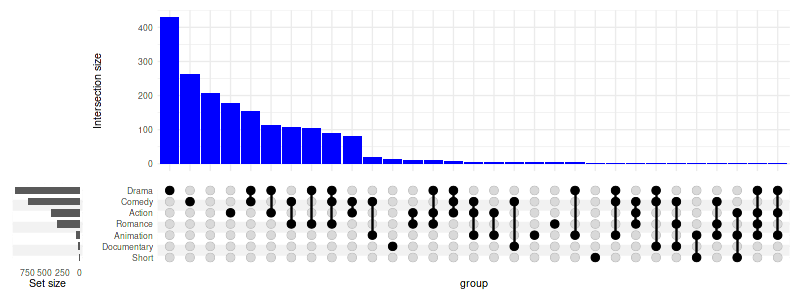
set_size(8, 3)

upset(
    movies,
    genres,
    base_annotations=list(
        'Intersection size'=intersection_size(
            counts=FALSE,
            mapping=aes(fill='bars_color')
        ) + scale_fill_manual(values=c('bars_color'='blue'), guide='none')
    ),
    width_ratio=0.1
)
3.3 Adjusting the height ratio
Setting height_ratio=1 will cause the intersection
matrix and the intersection size to have an equal height:
set_size(8, 3)

upset(
    movies,
    genres,
    height_ratio=1,
    width_ratio=0.1
)
3.6 Showing intersection size/union size ratio
It can be useful to visualise which intersections are larger than expected by chance (assuming equal probability of belonging to multiple sets); this can be achieved using the intersection size/union size ratio.
set_size(8, 6)
upset(
    movies, genres, name='genre', width_ratio=0.1, min_size=10,
    base_annotations=list(
        'Intersection size'=intersection_size(),
        'Intersection ratio'=intersection_ratio()
    )
)
Warning message:
“
[1m
[22mRemoved 62 rows containing missing values (`position_stack()`).”
The plot above tells us that the analysed documentary movies are almost always (in over 60% of cases) documentaries (and nothing more!), while comedies more often include elements of other genres (e.g. drama, romance) rather than being comedies alone (like stand-up shows).
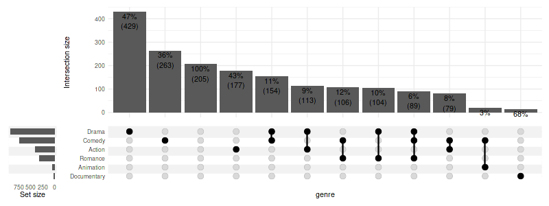
3.7 Showing percentages
text_mapping can be used to manipulate the aesthetics of
the labels. Using the intersection_size and
union_size one can calculate percentage of items in the
intersection (relative to the potential size of the intersection). A
upset_text_percentage(digits=0, sep='') shorthand is
provided for convenience:
set_size(8, 6)
upset(
    movies, genres, name='genre', width_ratio=0.1, min_size=10,
    base_annotations=list(
        # with manual aes specification:
        'Intersection size'=intersection_size(text_mapping=aes(label=paste0(round(
            !!get_size_mode('exclusive_intersection')/!!get_size_mode('inclusive_union') * 100
        ), '%'))),
        # using shorthand:
        'Intersection ratio'=intersection_ratio(text_mapping=aes(label=!!upset_text_percentage()))
    )
)
Warning message:
“
[1m
[22mRemoved 62 rows containing missing values (`position_stack()`).”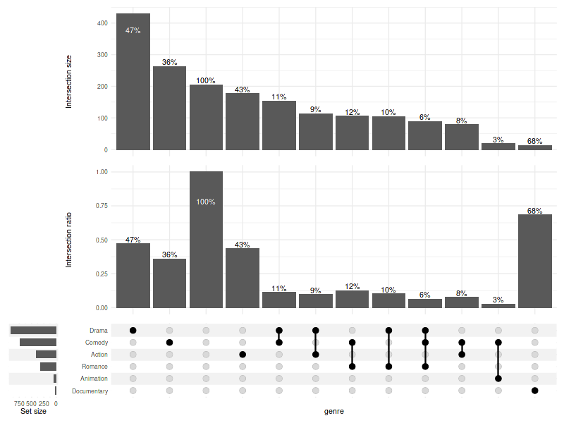
Also see 10. Display percentages.
3.7.1 Showing percentages and numbers together
set_size(8, 3)
upset(
    movies, genres, name='genre', width_ratio=0.1, min_size=10,
    base_annotations=list(
        'Intersection size'=intersection_size(
            text_mapping=aes(label=paste0(
                !!upset_text_percentage(),
                '\n',
                '(',
                !!get_size_mode('exclusive_intersection'),
                ')'
            )),
            bar_number_threshold=1,
            text=list(vjust=1.1)
        )
    )
)
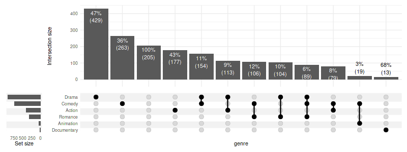
3.8 Custom positioning on bars/background
If adjusting bar_number_threshold is not sufficient, you
can specify custom rules for placement of text on bars/background:
set_size(8, 3)
size = get_size_mode('exclusive_intersection')
upset(
    movies, genres, name='genre', width_ratio=0.1, min_size=10,
    base_annotations=list(
        'Intersection size'=intersection_size(
            text_mapping=aes(
                label=paste0(
                    !!upset_text_percentage(),
                    '\n(', !!size, ')'
                ),
                colour=ifelse(!!size > 50, 'on_bar', 'on_background'),
                y=ifelse(!!size > 50, !!size - 100, !!size)
            )
        )
    )
)
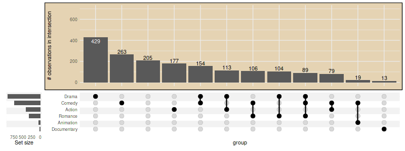
3.8 Further adjustments using ggplot2 functions
set_size(8, 3)
upset(
    movies, genres, width_ratio=0.1,
    base_annotations = list(
        'Intersection size'=(
            intersection_size()
            + ylim(c(0, 700))
            + theme(plot.background=element_rect(fill='#E5D3B3'))
            + ylab('# observations in intersection')
        )
    ),
    min_size=10
)
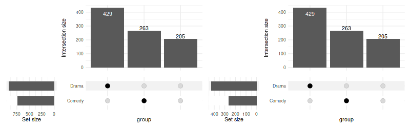
4. Adjusting “set size”
When using thresholding or selection criteria (such as
min_size or n_intersections) the change in
number of elements in each set size is not reflected in the set sizes
plot by default. You can change this by providing
filter_intersections=TRUE to
upset_set_size.
set_size(8, 2.5)
upset(
    movies, genres,
    min_size=200,
    set_sizes=upset_set_size()
) | upset(
    movies, genres,
    min_size=200,
    set_sizes=upset_set_size(filter_intersections=TRUE)
)
4.1 Rotate labels
To rotate the labels modify corresponding theme:
set_size(4, 3)
upset(
    movies, genres,
    min_size=100,
    width_ratio=0.15,
    set_sizes=(
        upset_set_size()
        + theme(axis.text.x=element_text(angle=90))
    )
)
To display the ticks:
set_size(4, 3)
upset(
    movies, genres, width_ratio=0.3, min_size=100,
    set_sizes=(
        upset_set_size()
        + theme(axis.ticks.x=element_line())
    )
)
4.2 Modify geoms and other layers
Arguments of the geom_bar can be adjusted in
upset_set_size; it can use a different geom, or be replaced
with a custom list of layers altogether:
set_size(8, 3)

(
    upset(
        movies, genres, width_ratio=0.5, max_size=100, min_size=15, wrap=TRUE,
        set_sizes=upset_set_size(
            geom=geom_bar(width=0.4)
        )
    )
    +
    upset(
        movies, genres, width_ratio=0.5, max_size=100, min_size=15, wrap=TRUE,
        set_sizes=upset_set_size(
            geom=geom_point(
                stat='count',
                color='blue'
            )
        )
    )
    +
    upset(
        movies, genres, width_ratio=0.5, max_size=100, min_size=15, wrap=TRUE,
        set_sizes=(
            upset_set_size(
                geom=geom_point(stat='count'),
                mapping=aes(y=..count../max(..count..)),
            )
            + ylab('Size relative to the largest')
        )
    )
)
Warning message:
“
[1m
[22mThe dot-dot notation (`..count..`) was deprecated in ggplot2 3.4.0.
[36mℹ
[39m Please use `after_stat(count)` instead.
[36mℹ
[39m The deprecated feature was likely used in the
[34mComplexUpset
[39m package.
Please report the issue at
[3m
[34m<https://github.com/krassowski/complex-upset/issues>
[39m
[23m.”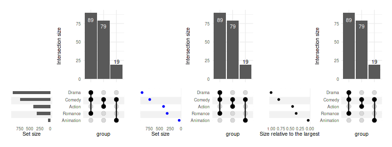
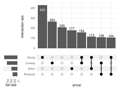
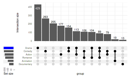
4.3 Logarithmic scale
In order to use a log scale we need to pass additional scale to in
layers argument. However, as the bars are on flipped
coordinates, we need a reversed log transformation. Appropriate
function, reverse_log_trans() is provided:
set_size(5, 3)

upset(
    movies, genres,
    width_ratio=0.1,
    min_size=10,
    set_sizes=(
        upset_set_size()
        + theme(axis.text.x=element_text(angle=90))
        + scale_y_continuous(trans=reverse_log_trans())
    ),
    queries=list(upset_query(set='Drama', fill='blue'))
)
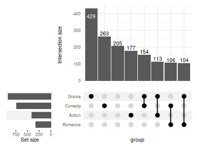
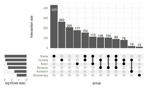
We can also modify the labels to display the logged values:
set_size(5, 3)

upset(
    movies, genres,
    min_size=10,
    width_ratio=0.2,
    set_sizes=upset_set_size()
        + scale_y_continuous(
            trans=reverse_log_trans(),
            labels=log10
        )
        + ylab('log10(set size)')
)
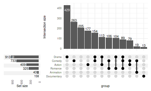
4.4 Display counts
To display the count add geom_text():
set_size(5, 3)

upset(
    movies, genres,
    min_size=10,
    width_ratio=0.3,
    encode_sets=FALSE,  # for annotate() to select the set by name disable encoding
    set_sizes=(
        upset_set_size()
        + geom_text(aes(label=..count..), hjust=1.1, stat='count')
        # you can also add annotations on top of bars:
        + annotate(geom='text', label='@', x='Drama', y=850, color='white', size=3)
        + expand_limits(y=1100)
        + theme(axis.text.x=element_text(angle=90))
    )
)
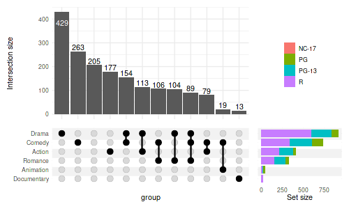
4.5 Change position and add fill
set_size(5, 3)

upset(
    movies, genres,
    min_size=10,
    width_ratio=0.3,
    set_sizes=(
        upset_set_size(
            geom=geom_bar(
                aes(fill=mpaa, x=group),
                width=0.8
            ),
            position='right'
        )
    ),
    # moves legends over the set sizes
    guides='over'
)
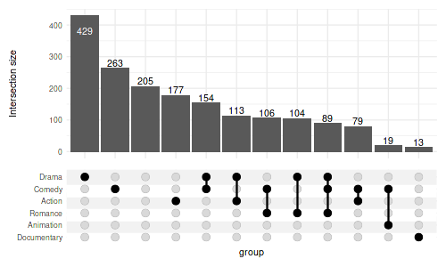
4.6 Hide the set sizes altogether
set_size(5, 3)

upset(
    movies, genres,
    min_size=10,
    set_sizes=FALSE
)
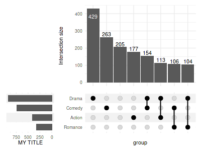
4.7 Change the label
For compatibility with older ggplot2 versions,
upset_set_size generates a plot with flipped coordinates
and therefore ylab needs to be used instead of
xlab (and aesthetic x is used in examples
above in place of y. This wil change it in a future major
release of ComplexUpset.
set_size(4, 3)
upset(
    movies, genres, width_ratio=0.3, min_size=100,
    set_sizes=(
        upset_set_size()
        + ylab('MY TITLE')
    )
)
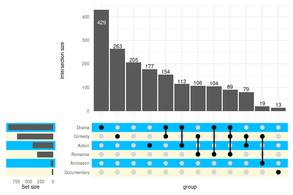
5. Adjusting other aesthetics
5.1 Stripes
Change the colors:
set_size(6, 4)
upset(
    movies,
    genres,
    min_size=10,
    width_ratio=0.2,
    stripes=c('cornsilk1', 'deepskyblue1')
)
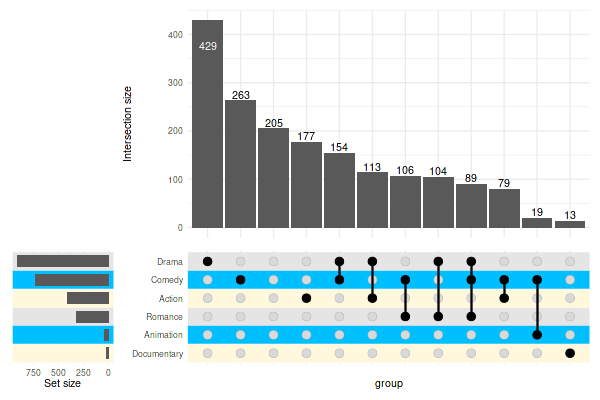
You can use multiple colors:
set_size(6, 4)
upset(
    movies,
    genres,
    min_size=10,
    width_ratio=0.2,
    stripes=c('cornsilk1', 'deepskyblue1', 'grey90')
)
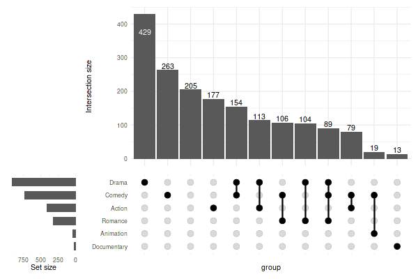
Or, set the color to white to effectively disable the stripes:
set_size(6, 4)
upset(
    movies,
    genres,
    min_size=10,
    width_ratio=0.2,
    stripes='white'
)
Advanced customization using upset_stripes():
set_size(6, 4)
upset(
    movies,
    genres,
    min_size=10,
    width_ratio=0.2,
    stripes=upset_stripes(
        geom=geom_segment(size=5),
        colors=c('cornsilk1', 'deepskyblue1', 'grey90')
    )
)
Warning message:
“
[1m
[22mUsing `size` aesthetic for lines was deprecated in ggplot2 3.4.0.
[36mℹ
[39m Please use `linewidth` instead.”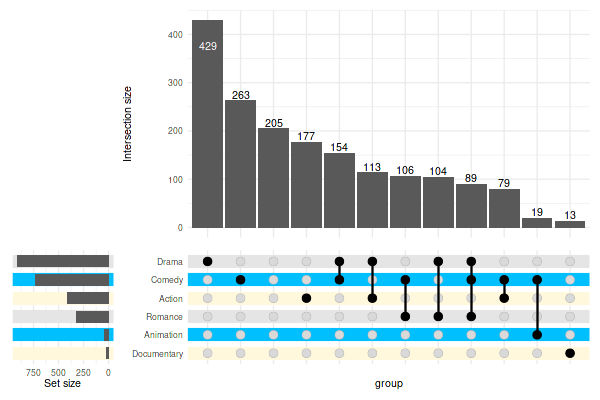
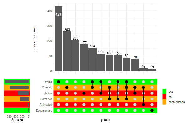
Mapping stripes attributes to data using
upset_stripes():
set_size(6, 4)
genre_metadata = data.frame(
    set=c('Action', 'Animation', 'Comedy', 'Drama', 'Documentary', 'Romance', 'Short'),
    shown_in_our_cinema=c('no', 'no', 'on weekends', 'yes', 'yes', 'on weekends', 'no')
)

upset(
    movies,
    genres,
    min_size=10,
    width_ratio=0.2,
    stripes=upset_stripes(
        mapping=aes(color=shown_in_our_cinema),
        colors=c(
            'yes'='green',
            'no'='red',
            'on weekends'='orange'
        ),
        data=genre_metadata
    )
)
5.2 Adding title
Adding title with ggtitle with add it to the
intersection matrix:
In order to add a title for the entire plot, you need to wrap the plot:
set_size(6, 4)
upset(movies, genres, min_size=10, wrap=TRUE) + ggtitle('The overlap between genres')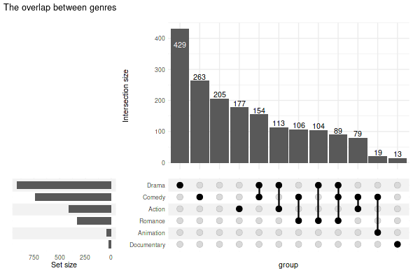
5.3 Making the plot transparent
You need to set the plot background to transparent and adjust colors of stripes to your liking:
set_size(6, 4)
(
    upset(
        movies, genres, name='genre', width_ratio=0.1, min_size=10,
        stripes=c(alpha('grey90', 0.45), alpha('white', 0.3))
    )
    & theme(plot.background=element_rect(fill='transparent', color=NA))
)
Use ggsave('upset.png', bg="transparent") when exporting
to PNG.
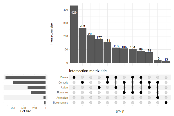
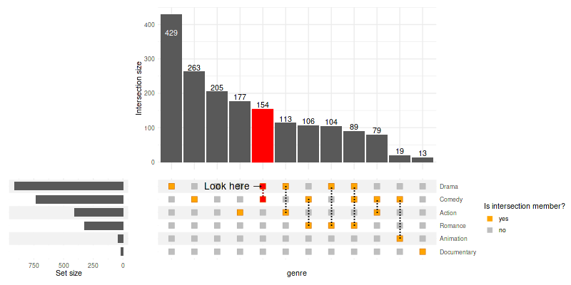
5.4 Adjusting the intersection matrix
Use intersection_matrix() to modify the matrix
parameters:
set_size(8, 4)
upset(
    movies, genres, name='genre', min_size=10,
    encode_sets=FALSE,  # for annotate() to select the set by name disable encoding
    matrix=(
        intersection_matrix(
            geom=geom_point(
                shape='square',
                size=3.5
            ),
            segment=geom_segment(
                linetype='dotted'
            ),
            outline_color=list(
                active='darkorange3',
                inactive='grey70'
            )
        )
        + scale_color_manual(
            values=c('TRUE'='orange', 'FALSE'='grey'),
            labels=c('TRUE'='yes', 'FALSE'='no'),
            breaks=c('TRUE', 'FALSE'),
            name='Is intersection member?'
        )
        + scale_y_discrete(
            position='right'
        )
        + annotate(
            geom='text',
            label='Look here →',
            x='Comedy-Drama',
            y='Drama',
            size=5,
            hjust=1
        )
    ),
    queries=list(
        upset_query(
            intersect=c('Drama', 'Comedy'),
            color='red',
            fill='red',
            only_components=c('intersections_matrix', 'Intersection size')
        )
    )
)
6. Themes
The themes for specific components are defined in
upset_themes list, which contains themes for:
names(upset_themes)- ‘intersections_matrix’
- ‘Intersection size’
- ‘overall_sizes’
- ‘default’
You can substitute this list for your own using themes
argument. While you can specify a theme for every component, if you omit
one or more components those will be taken from the element named
default.
6.1 Substituting themes
You can also add themes for your custom panels/annotations:
set_size(8, 8)

upset(
    movies,
    genres,
    annotations = list(
        'Length'=list(
            aes=aes(x=intersection, y=length),
            geom=geom_boxplot(na.rm=TRUE)
        ),
        'Rating'=list(
            aes=aes(x=intersection, y=rating),
            geom=list(
                geom_jitter(aes(color=log10(votes)), na.rm=TRUE),
                geom_violin(alpha=0.5, na.rm=TRUE)
            )
        )
    ),
    min_size=10,
    width_ratio=0.1,
    themes=modifyList(
        upset_themes,
        list(Rating=theme_void(), Length=theme())
    )
)
6.2 Adjusting the default themes
Modify all the default themes as once with
upset_default_themes():
set_size(8, 4)

upset(
    movies, genres, min_size=10, width_ratio=0.1,
    themes=upset_default_themes(text=element_text(color='red'))
)
To modify only a subset of default themes use
upset_modify_themes():
set_size(8, 4)

upset(
    movies, genres,
    base_annotations=list('Intersection size'=intersection_size(counts=FALSE)),
    min_size=100,
    width_ratio=0.1,
    themes=upset_modify_themes(
        list(
            'intersections_matrix'=theme(text=element_text(size=20)),
            'overall_sizes'=theme(axis.text.x=element_text(angle=90))
        )
    )
)
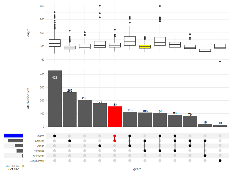
7. Highlighting (queries)
Pass a list of lists generated with upset_query()
utility to the optional queries argument to selectively
modify aesthetics of specific intersections or sets.
Use one of the arguments: set or intersect
(not both) to specify what to highlight: - set will
highlight the bar of the set size, - intersect will
highlight an intersection on all components (by default), or on
components chosen with only_components - all other
parameters will be used to modify the geoms
set_size(8, 6)

upset(
    movies, genres, name='genre', width_ratio=0.1, min_size=10,
    annotations = list(
        'Length'=list(
            aes=aes(x=intersection, y=length),
            geom=geom_boxplot(na.rm=TRUE)
        )
    ),
    queries=list(
        upset_query(
            intersect=c('Drama', 'Comedy'),
            color='red',
            fill='red',
            only_components=c('intersections_matrix', 'Intersection size')
        ),
        upset_query(
            set='Drama',
            fill='blue'
        ),
        upset_query(
            intersect=c('Romance', 'Comedy'),
            fill='yellow',
            only_components=c('Length')
        )
    )
)
8. Sorting
8.1 Sorting intersections
By degree:
set_size(8, 3)
upset(movies, genres, width_ratio=0.1, sort_intersections_by='degree')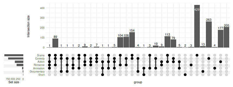
By ratio:
set_size(8, 4)
upset(
    movies, genres, name='genre', width_ratio=0.1, min_size=10,
    sort_intersections_by='ratio',
    base_annotations=list(
        'Intersection size'=intersection_size(text_mapping=aes(label=!!upset_text_percentage())),
        'Intersection ratio'=intersection_ratio(text_mapping=aes(label=!!upset_text_percentage()))
    )
)
Warning message:
“
[1m
[22mRemoved 62 rows containing missing values (`position_stack()`).”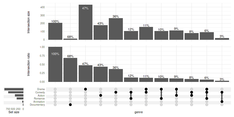
The other way around:
set_size(8, 3)
upset(movies, genres, width_ratio=0.1, sort_intersections='ascending')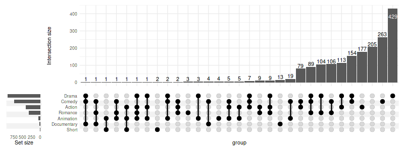
Without any sorting:
set_size(8, 3)
upset(movies, genres, width_ratio=0.1, sort_intersections=FALSE)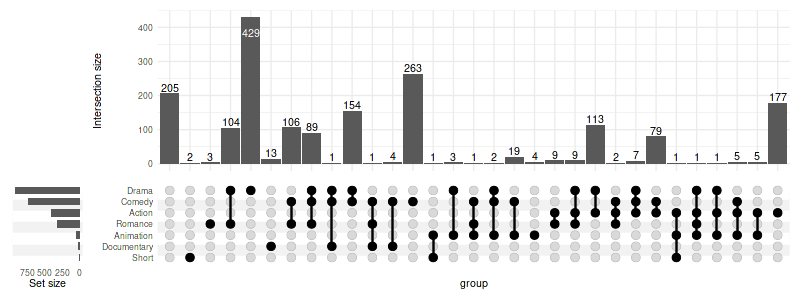
First by degree then by cardinality:
set_size(8, 3)
upset(movies, genres, width_ratio=0.1, sort_intersections_by=c('degree', 'cardinality'))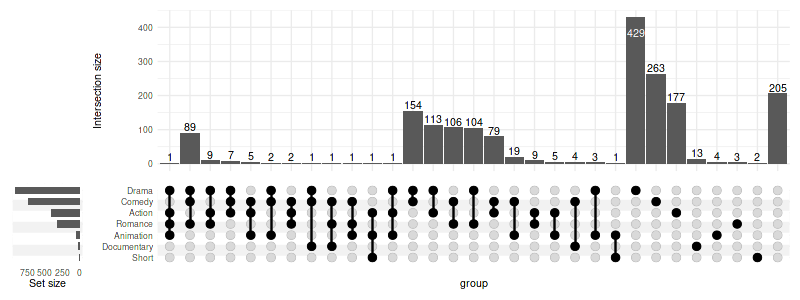
User-specified order:
set_size(6, 3)
upset(
    movies,
    genres,
    width_ratio=0.1,
    sort_intersections=FALSE,
    intersections=list(
        'Comedy',
        'Drama',
        c('Comedy', 'Romance'),
        c('Romance', 'Drama'),
        'Outside of known sets',
        'Action'
    )
)
8.2 Sorting sets
Ascending:
set_size(8, 3)
upset(movies, genres, width_ratio=0.1, sort_sets='ascending')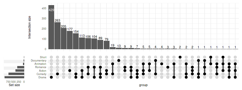
Without sorting - preserving the order as in genres:
genres- ‘Action’
- ‘Animation’
- ‘Comedy’
- ‘Drama’
- ‘Documentary’
- ‘Romance’
- ‘Short’
set_size(8, 3)
upset(movies, genres, width_ratio=0.1, sort_sets=FALSE)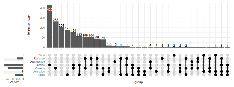
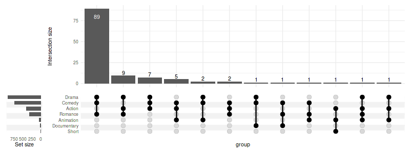
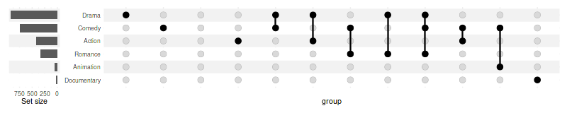
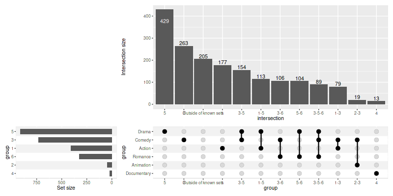
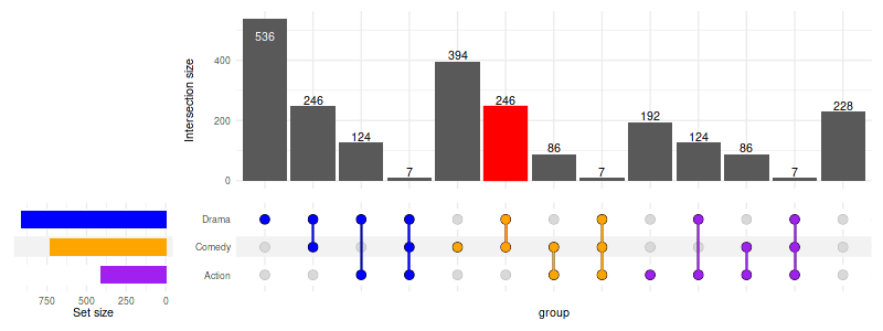
9. Grouping
9.1 Grouping intersections
Use group_by='sets' to group intersections by set. If
needed, the intersections will be repeated so that they appear in each
set group. Use upset_query() with group
argument to color the intersection matrix accordingly.
set_size(8, 3)

upset(
    movies, c("Action", "Comedy", "Drama"),
    width_ratio=0.2,
    group_by='sets',
    queries=list(
        upset_query(
            intersect=c('Drama', 'Comedy'),
            color='red',
            fill='red',
            only_components=c('intersections_matrix', 'Intersection size')
        ),
        upset_query(group='Drama', color='blue'),
        upset_query(group='Comedy', color='orange'),
        upset_query(group='Action', color='purple'),
        upset_query(set='Drama', fill='blue'),
        upset_query(set='Comedy', fill='orange'),
        upset_query(set='Action', fill='purple')
    )
)
10. Display percentages
Use aes_percentage() utility preceded with
!! syntax to easily display percentages. In the examples
below only percentages for the movies with R rating are shown to avoid
visual clutter.
rating_scale = scale_fill_manual(values=c(
    'R'='#E41A1C', 'PG'='#377EB8',
    'PG-13'='#4DAF4A', 'NC-17'='#FF7F00'
))
show_hide_scale = scale_color_manual(values=c('show'='black', 'hide'='transparent'), guide='none')
10.1 Within intersection
set_size(8, 5)

upset(
    movies, genres, name='genre', width_ratio=0.1, min_size=100,
    annotations =list(
        'MPAA Rating'=list(
            aes=aes(x=intersection, fill=mpaa),
            geom=list(
                geom_bar(stat='count', position='fill', na.rm=TRUE),
                geom_text(
                    aes(
                        label=!!aes_percentage(relative_to='intersection'),
                        color=ifelse(mpaa == 'R', 'show', 'hide')
                    ),
                    stat='count',
                    position=position_fill(vjust = .5)
                ),
                scale_y_continuous(labels=scales::percent_format()),
                show_hide_scale,
                rating_scale
            )
        )
    )
)
Warning message:
“
[1m
[22mRemoved 262 rows containing non-finite values (`stat_count()`).”
10.2 Relative to the group
set_size(8, 5)

upset(
    movies, genres, name='genre', width_ratio=0.1, min_size=100,
    annotations =list(
        'MPAA Rating'=list(
            aes=aes(x=intersection, fill=mpaa),
            geom=list(
                geom_bar(stat='count', position='fill', na.rm=TRUE),
                geom_text(
                    aes(
                        label=!!aes_percentage(relative_to='group'),
                        group=mpaa,
                        color=ifelse(mpaa == 'R', 'show', 'hide')
                    ),
                    stat='count',
                    position=position_fill(vjust = .5)
                ),
                scale_y_continuous(labels=scales::percent_format()),
                show_hide_scale,
                rating_scale
            )
        )
    )
)
Warning message:
“
[1m
[22mRemoved 262 rows containing non-finite values (`stat_count()`).”
10.3 Relative to all observed values
set_size(8, 5)

upset(
    movies, genres, name='genre', width_ratio=0.1, min_size=100,
    annotations =list(
        'MPAA Rating'=list(
            aes=aes(x=intersection, fill=mpaa),
            geom=list(
                geom_bar(stat='count', position='fill', na.rm=TRUE),
                geom_text(
                    aes(
                        label=!!aes_percentage(relative_to='all'),
                        color=ifelse(mpaa == 'R', 'show', 'hide')
                    ),
                    stat='count',
                    position=position_fill(vjust = .5)
                ),
                scale_y_continuous(labels=scales::percent_format()),
                show_hide_scale,
                rating_scale
            )
        )
    )
)
Warning message:
“
[1m
[22mRemoved 262 rows containing non-finite values (`stat_count()`).”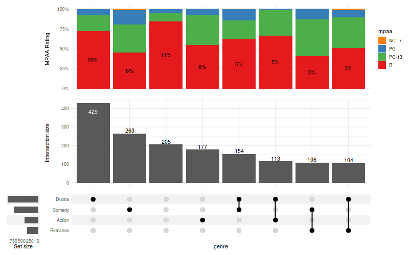
11. Advanced usage examples
11.1 Display text on some bars only
set_size(8, 5)

upset(
    movies, genres, name='genre', width_ratio=0.1, min_size=100,
    annotations =list(
        'MPAA Rating'=list(
            aes=aes(x=intersection, fill=mpaa),
            geom=list(
                geom_bar(stat='count', position='fill', na.rm=TRUE),
                geom_text(
                    aes(label=ifelse(mpaa == 'R', 'R', NA)),
                    stat='count',
                    position=position_fill(vjust = .5),
                    na.rm=TRUE
                ),
                show_hide_scale,
                rating_scale
            )
        )
    )
)
11.2 Combine multiple plots together
set_size(8, 5)
library(patchwork)

annotations = list(
    'MPAA Rating'=list(
        aes=aes(x=intersection, fill=mpaa),
        geom=list(
            geom_bar(stat='count', position='fill')
        )
    )
)
set.seed(0)    # for replicable example only

data_1 = movies[sample(nrow(movies), 100), ]
data_2 = movies[sample(nrow(movies), 100), ]

u1 = upset(data_1, genres, min_size=5, base_annotations=annotations)
u2 = upset(data_2, genres, min_size=5, base_annotations=annotations)

(u1 | u2) + plot_layout(guides='collect')
Warning message:
“
[1m
[22mRemoved 16 rows containing non-finite values (`stat_count()`).”
Warning message:
“
[1m
[22mRemoved 15 rows containing non-finite values (`stat_count()`).”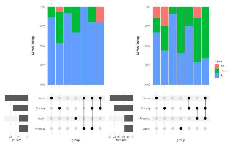
11.3 Change height of the annotations
set_size(8, 3.5)
upset(
    movies, genres, name='genre', width_ratio=0.1, min_size=100,
    annotations =list(
        'MPAA Rating'=list(
            aes=aes(x=intersection, fill=mpaa),
            geom=list(
                geom_bar(stat='count', position='fill'),
                scale_y_continuous(labels=scales::percent_format())
            )
        )
    )
) + patchwork::plot_layout(heights=c(0.5, 1, 0.5))
Warning message:
“
[1m
[22mRemoved 262 rows containing non-finite values (`stat_count()`).”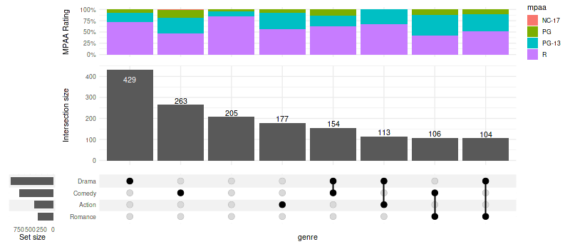
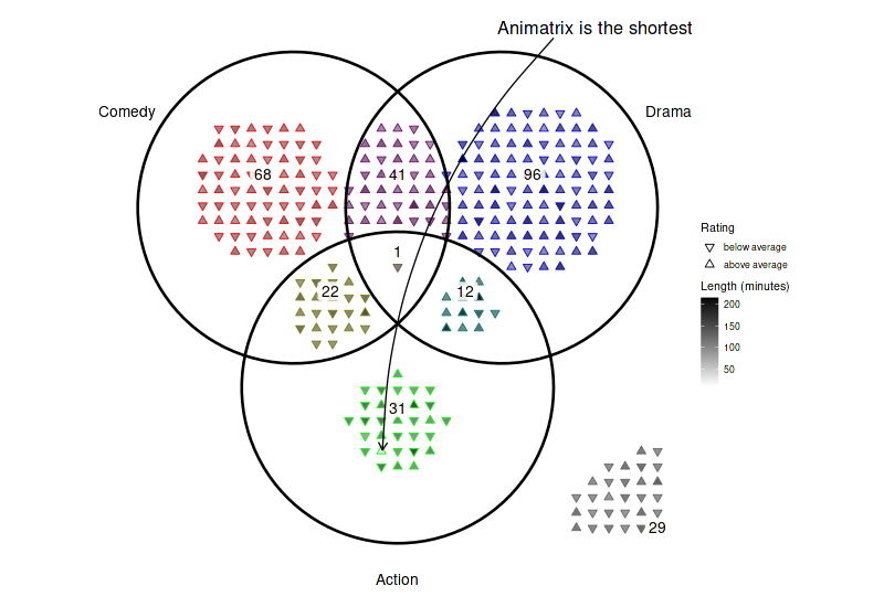
12. Venn diagrams
Simple implementation of Venn diagrams is provided, taking the same
input format as upset() but only supporting up to three
sets.
movies_subset = head(movies, 300)
genres_subset = c('Comedy', 'Drama', 'Action')

movies_subset$good_rating = movies_subset$rating > mean(movies_subset$rating)
arranged = arrange_venn(movies_subset, sets=genres_subset)
12.1 Highlight specific elements
set_size(8, 5.5)
(
    ggplot(arranged)
    + theme_void()
    + coord_fixed()
    + geom_point(aes(x=x, y=y, color=region, shape=good_rating, fill=length), size=2.7)
    + geom_venn_circle(movies_subset, sets=genres_subset, size=1)
    + geom_venn_label_set(movies_subset, sets=genres_subset, aes(label=region), outwards_adjust=2.6)
    + geom_venn_label_region(movies_subset, sets=genres_subset, aes(label=size), position=position_nudge(y=0.15))
    + geom_curve(
        data=arranged[which.min(arranged$length), ],
        aes(xend=x+0.01, yend=y+0.01), x=1.5, y=2.5, curvature=.2,
        arrow = arrow(length = unit(0.015, "npc"))
    )
    + annotate(
        geom='text', x=1.9, y=2.6, size=6,
        label=paste(substr(arranged[which.min(arranged$length), ]$title, 0, 9), 'is the shortest')
    )
    + scale_color_venn_mix(movies, sets=genres_subset, guide='none')
    + scale_shape_manual(
        values=c(
            'TRUE'='triangle filled',
            'FALSE'='triangle down filled'
        ),
        labels=c(
            'TRUE'='above average',
            'FALSE'='below average'
        ),
        name='Rating'
    )
    + scale_fill_gradient(low='white', high='black', name='Length (minutes)')

)
12.2 Highlight all regions
set_size(8, 5.5)
(
    ggplot(arranged)
    + theme_void()
    + coord_fixed()
    + geom_venn_region(movies_subset, sets=genres_subset, alpha=0.1)
    + geom_point(aes(x=x, y=y, color=region), size=2.5)
    + geom_venn_circle(movies_subset, sets=genres_subset, size=1.5)
    + geom_venn_label_set(movies_subset, sets=genres_subset, aes(label=region), outwards_adjust=2.6)
    + geom_venn_label_region(movies_subset, sets=genres_subset, aes(label=size), position=position_nudge(y=0.15))
    + scale_color_venn_mix(movies, sets=genres_subset, guide='none')
    + scale_fill_venn_mix(movies, sets=genres_subset, guide='none')
)
12.3 Highlight specific regions
set_size(8, 5.5)

(
    ggplot(arranged)
    + theme_void()
    + coord_fixed()
    + geom_venn_region(movies_subset, sets=genres_subset, alpha=0.2)
    + geom_point(aes(x=x, y=y, color=region), size=1.5)
    + geom_venn_circle(movies_subset, sets=genres_subset, size=2)
    + geom_venn_label_set(movies_subset, sets=genres_subset, aes(label=region), outwards_adjust=2.6)
    + scale_color_venn_mix(movies, sets=genres_subset, guide='none')
    + scale_fill_venn_mix(movies, sets=genres_subset, guide='none', highlight=c('Comedy-Action', 'Drama'), inactive_color='white')
)
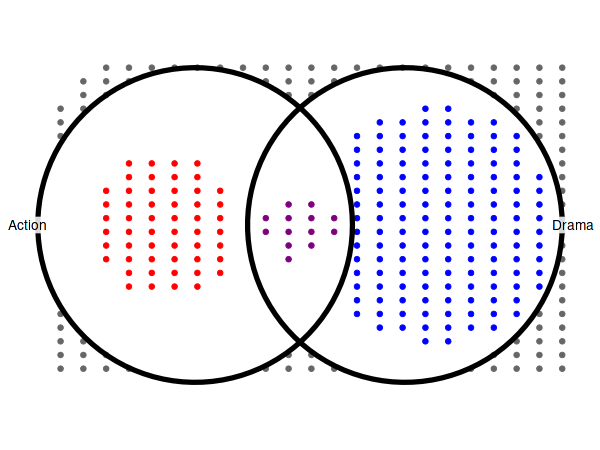
12.4 Two sets Venn
The density of the points grid is determined in such a way that the all the points from the set with the largest space restrictions are fit into the available area. In case of the diagram below, its the observations that do not belong to any set that define the grid density:
set_size(6, 4.5)
genres_subset = c('Action', 'Drama')
(
    ggplot(arrange_venn(movies_subset, sets=genres_subset))
    + theme_void()
    + coord_fixed()
    + geom_point(aes(x=x, y=y, color=region), size=2)
    + geom_venn_circle(movies_subset, sets=genres_subset, size=2)
    + geom_venn_label_set(movies_subset, sets=genres_subset, aes(label=region), outwards_adjust=2.6)
    + scale_color_venn_mix(movies, sets=genres_subset, guide='none')
)